Tutorial 1: Basic Reconstructions
This tutorial will guide you through the first simple tomography reconstruction. By the end, you will be able to:
Load a set of projection images
Produce a single reconstructed slice
Produce the full reconstructed volume
Supply command line arguments to alter the reconstruction behavior
Create a configuration file to stream-line reconstructions
Note
This tutorial assumes you have a working python installation (i.e. Anaconda) and have installed tomopy-cli and it’s dependencies (both tomopy and dxchange).
Warning
This tutorial has only been tested on GNU/Linux operating systems. Windows and MacOS support is an ongoing project.
Preamble: Prepare Test Images
Note
This tutorial will use some test data known as the Shepp-Logan phantom, which will need to be saved in a format that mimics synchrotron tomography data. This preamble section is not needed when performing reconstructions on real experimental data.
First, open a terminal and create an empty directory to hold our data:
$ mkdir tomopy_cli_tutorial
$ cd tomopy_cli_tutorial
We will also need a way to view the results of our reconstruction, so we’ll install matplotlib:
$ pip install matplotlib
Now open a python console ($ python) and use the tomopy
package to prepare phantom test data:
>>> import tomopy, dxchange, numpy, h5py, matplotlib.pyplot as plt
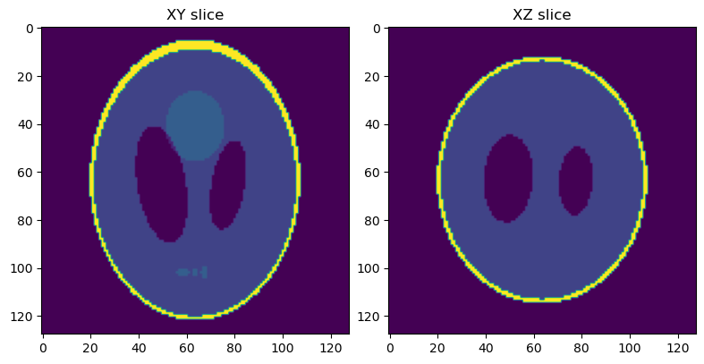
>>> phantom = tomopy.misc.phantom.shepp3d(128)
And visualize the results:
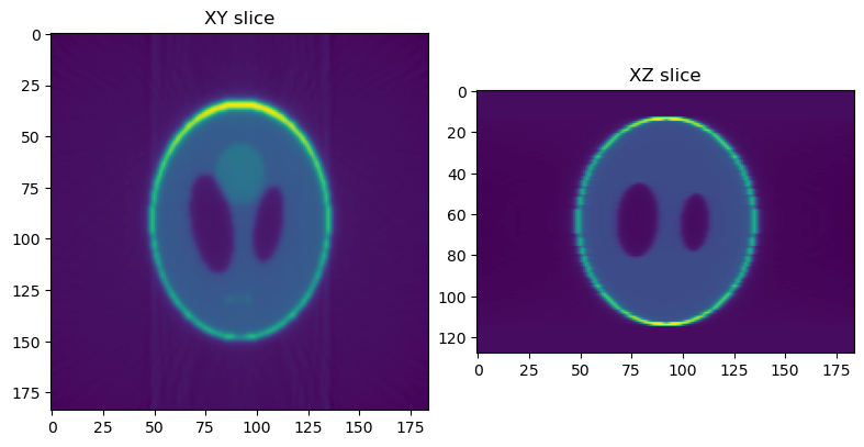
>>> fig, (axL, axR) = plt.subplots(1, 2)
>>> axL.imshow(phantom[64])
>>> axL.set_title("XY slice")
>>> axR.imshow(phantom[:,64])
>>> axR.set_title("XZ slice")
>>> plt.show(block=False)
You should now see a plot with a horizontal (XY) slice and a vertical (XZ) slice of the test data:
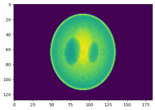
Next, we will simulate a set of projection images from this phantom volume.
>>> angles = tomopy.sim.project.angles(181)
>>> proj = tomopy.sim.project.project(phantom, theta=angles)
>>> plt.figure()
>>> plt.imshow(proj[0])
>>> plt.show(block=False)
You should now see the first image in a series of simulated projections of the phantom volume.
This set of projections will be used as input for reconstructions in the rest of this tutorial, so we will save them and then leave the python console for the next segment of this tutorial:
Warning
This following commands will overwrite any existing file named phantom_projections.h5.
>>> file = h5py.File("phantom_projections.h5", mode="w")
>>> file.create_dataset("exchange/data", data=numpy.exp(-proj))
>>> file.create_dataset("exchange/data_white", data=numpy.ones(shape=(1, *proj.shape[-2:])))
>>> file.create_dataset("exchange/data_dark", data=numpy.zeros(shape=(1, *proj.shape[-2:])))
>>> file.close()
>>> exit()
Perform a Single Slice Reconstruction
Now that we have some projection data work with, we will perform a simple single-slice reconstruction:
$ tomopy recon --file-name phantom_projections.h5 --reconstruction-type=slice --output-folder=_rec
This will save reconstructions as TIFF files in the _rec folder. Single slice reconstructions are stored in _rec/slice_rec.
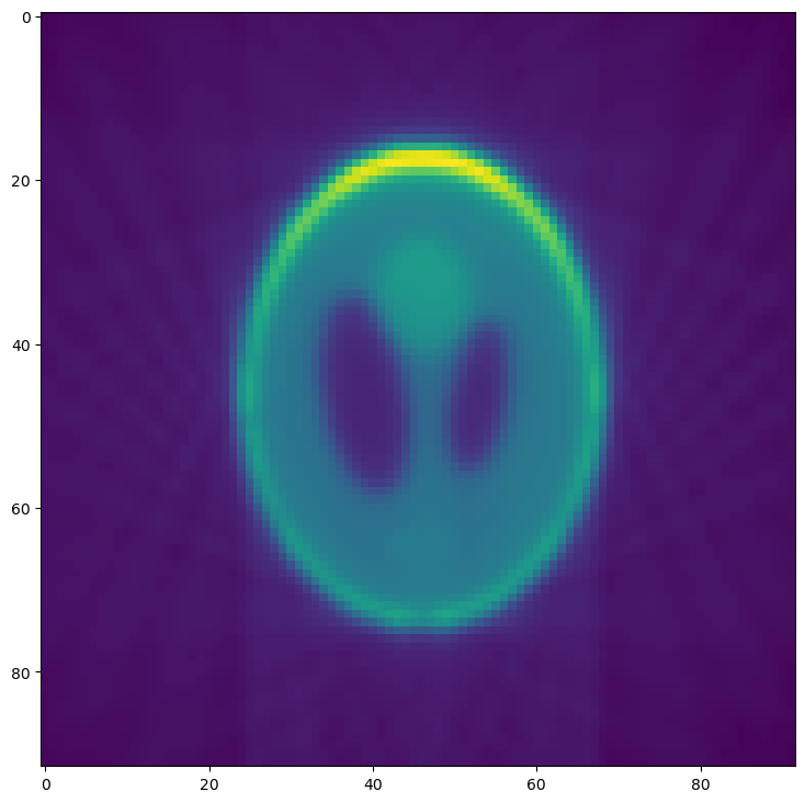
To visualize the results, open a python console again and use matplotlib to view the reconstructed data.
>>> import matplotlib.pyplot as plt, imageio
>>> slc = imageio.read("_rec/slice_rec/recon_phantom_projections.tiff").get_data(0)
>>> plt.figure()
>>> plt.imshow(slc)
>>> plt.show(block=False)
Compare this reconstructed slice to the original phantom produced in the first section.
Perform a Full Volume Reconstruction
We will now use tomopy-cli to reconstruct the full volume. This is
done by changing the --reconstruction-type option:
$ tomopy recon --file-name phantom_projections.h5 --reconstruction-type=full --output-folder=_rec --output-format=tiff_stack
Reconstructions are again stored in _rec, but full volume reconstructions can be found in _rec/phantom_projections_rec. Again, open a python console to visualize the results:
>>> import matplotlib.pyplot as plt, dxchange
>>> recon = dxchange.read_tiff_stack("_rec/phantom_projections_rec/recon_00000.tiff", ind=range(0, 128))
>>> fig, (axL, axR) = plt.subplots(1, 2)
>>> axL.imshow(recon[64])
>>> axL.set_title("XY slice")
>>> axR.imshow(recon[:,92])
>>> axR.set_title("XZ slice")
>>> plt.show(block=False)
Modify Reconstruction Behavior
Now we will use some of tomopy-cli’s command line options to modify the reconstruction behavior. We will add four features to our reconstruction:
Downsample (bin) the data by a factor of 2
Manually specify the rotation center
Remove any NaN or infinity values
$ tomopy recon --file-name phantom_projections.h5 --reconstruction-type=slice --output-folder=_rec --binning=1 --rotation-axis-auto=manual --rotation-axis=91.5 --fix-nan-and-inf --fix-nan-and-inf-value=34.05
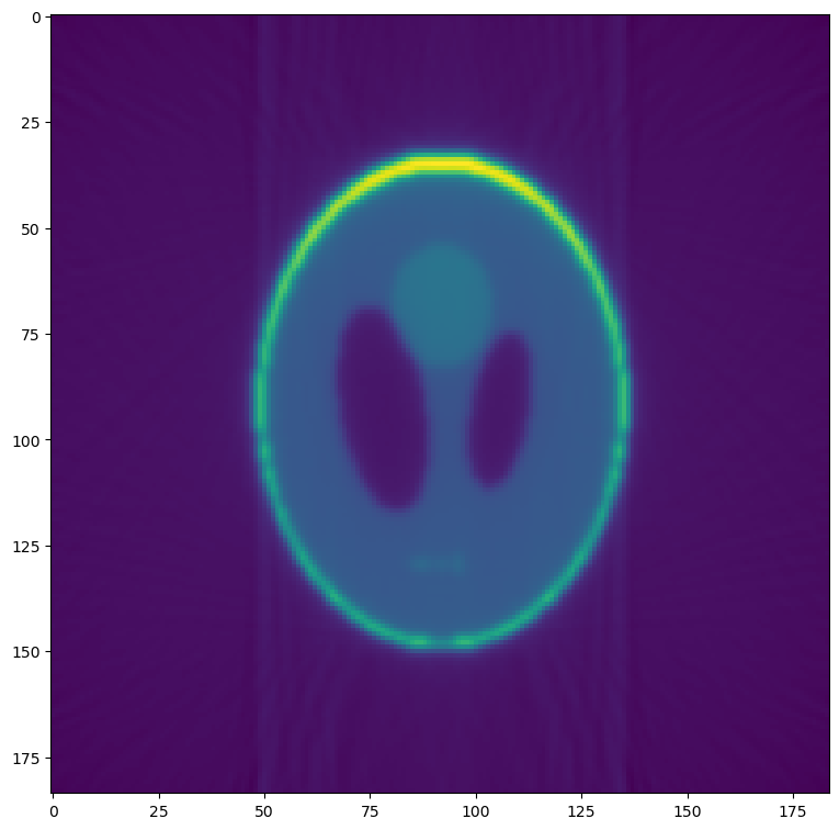
Now we will visualize the new reconstruction. Open a python console again and use matplotlib to view the reconstructed data.
Note
If you ran the previous slice reconstruction command more than once, you may have to modify the file name in the example below, since each time tomopy is run, a new tiff file is saved.
In this case, if the previous command was run twice, this would create files recon_phantom_projections.tiff and recon_phantom_projections-1.tiff, so we would now need to replace the file name with recon_phantom_projections-2.tiff
>>> import matplotlib.pyplot as plt, imageio
>>> slc = imageio.read("_rec/slice_rec/recon_phantom_projections-1.tiff").get_data(0)
>>> plt.figure()
>>> plt.imshow(slc)
>>> plt.show(block=False)
Comparing this reconstruction with the previous versions, the major
difference is the lower resolution and noise resulting from the
--binning=1 option. Since we are using well-behaved test data, the
other options have no noticeable effect.
Details for these options and many more can be seen by running
tomopy recon --help from the command line.